Convolution is just Matrix Multiplication

Hat tip to Penny at her excellent blog. The concepts and images referenced in this article are largely sourced from her work.

I was trying to understand how convolution is performed in GPU hardware and Penny gave me some good insights which inspired my own interpretation.

The computational process involved in training convolutional networks closely resembles matrix multiplication, exhibiting both intensive computation and high parallelism.

convolution == 2d dot product == unrolled 1d dot product == matrix multiplication

Penny says: “Thinking about it - convolution is just a 2d dot product”. This is a pretty useful analogy. However, 2D convolution and matrix products look quite different at first glance. One helpful insight is to note that all matrices and images are ultimately stored as flattened blocks of memory in our computing devices.

Example 3D Tensor Convolution

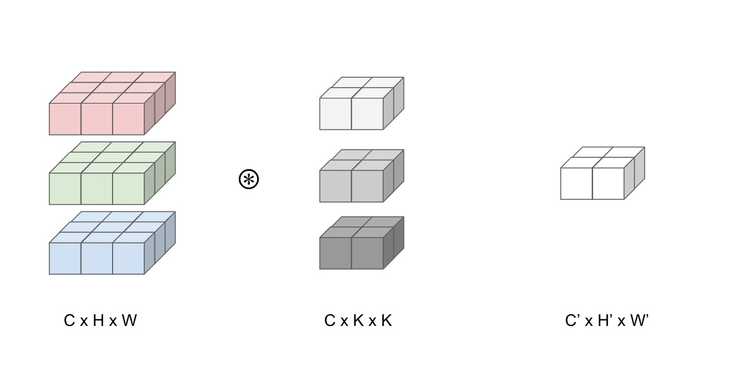
We present a 3D tensor convolution as a case in point. The simple illustration portrays the convolution of a 3x3x3 color image with a 3x2x2 kernel, resulting in a 2x2 activation layer. This convolution layer involves an input with 3 feature maps (input channel C = 3) of size 3x3, ultimately producing 1 feature map (output channel C’ = 1) of size 2x2.

    Input: C x H x W = (3 x 3 x 3)
    Kernel: C x K x K = (3 x 2 x 2)
    Output: C' H' x W' = (H - K + 1) x (W - K + 1) = (2 x 2)

So let’s see how we can express this 3D convolution as a Matrix Multiplication.

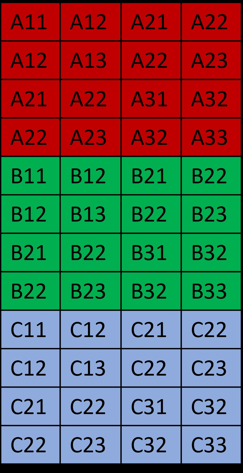
First notice how the both the input and the kernel is 3D. In order to use matrix multiplication, a conversion to 2D is necessary, necessitating the flattening of the kernel and the replication of the inputs, as shown below.

Reducing the input - the input elements needs to be rearranged and duplicated. Since the results of the convolutions are summed across input features, the input features can be concatenated into one large matrix. The height of the unrolled input equals the number of kernel elements, 12 in our case. The width of the unrolled input equals the number of output activations, which is 4 in our case.

Why is this Important?

These convolution layers and their calculation are the primary bottleneck in fast system applications. So to optimize these convolution layers, would you rather optimize a convolution or matrix multiplication? It turns out that it is much easier to tweak a matrix multiplication function in order to, say, optimize for speed or power through understanding the software implementation as well as how is it applied to hardware. In addition to optimizing the software through linear algebra libraries, recent areas of research are performed on specialized hardware, such as implementation on hardware accelerators to just do matrix multiplication. Indeed GPUs are specialized hardware which can do matrix multiplication in a very fast, parallelizable way.

Size Matters

One issue with the above construction is that the image size is increased from 27 elements to 36 elements while the kernel remains only 12 elements. The matrix appears as follows and there is a fair amount of redundancy in the image data. As images tend to be large and kernels tend to be small, it would make much more sense to have redundacy in the kernel representation instead of the image representation.

Here is another explanation from Baeldung which does it this way. Note that this is 2D convolution and not 3D.

Let’s say A (nxn) and K (mxm) are 3x3 and 2x2:

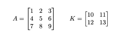
The corresponding convolution matrices are:

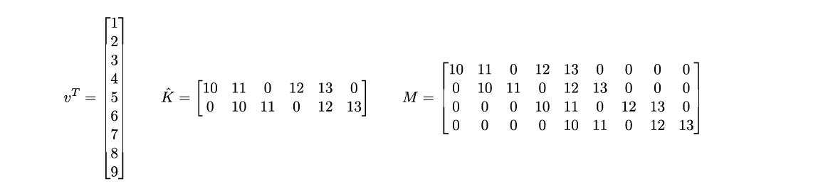
The result of this convolution is:

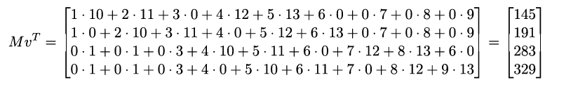
Here the image has the same number of elements but the kernel has increased from 4 elements to 36, which doesn’t look so good. In fact, if the image width is n=256 pixels, then M must have nxn=65,536 columns and (n-m)x(n-m)=64,516 rows. This is quite daunting. However note that M is a block circulant matrix. Each row is simply the same set of 4 elements shifted by either one or two columns in the example. This means we can replace the large M matrix by a simple vector of 4 elements representing the flattened kernel. Now it is simply a matter of calculating the dot product of the kernel vector with the image vector using pointers to shift the alignment of the kernel elements against the image vector. In this manner, neither the image nor the kernel is expanded in size and the task of convolution via matrix multiply reduces to set of simple vector dot products.

Enjoy!

I hope you now have a good idea of how deep learning convolutions can be expressed as matrices.

Brian